hercacstables
hercacstables.RmdWelcome
For the newest R users:
If you are new to R, but not data science, then I suggest checking out R for Data Science. If have a background that is not data science, then I have heard good things about this book.
First-time users of hercacstables
If this is your first time using this package then you probably want
to register with the Census. Registering is important because it helps
you make more queries to the API. The Census limits the number of
anonymous API queries that it receives from any one IP address. The
vignette("set_up_your_api_key") will guide you through the
process.
Otherwise, welcome back!
This package helps R users to access data from the United States Census Bureau, especially its American Community Survey.
The American Community Survey (ACS) from the US Census’s website provides a vast amount of useful data.
However, it returns those data in a weirdly idiosyncratic way. Even though the output seems tabular, the data are really organized in a tree-like fashion. This package is intended to make it easy to access and use the ACS data with R.
The database has an enormous amount of information, stored in a
versatile but cumbersome format. Data are stored in hundreds of
different tables, called “groups,” that give breakdowns of information.
For example, group B21005
reports counts of people according to their employment status, military
service, and age. Each row in a group reports a value for a specific
slice of the topic. For example, row 5 in group B21005
gives the number of employed veterans between the ages of 18 and 34. The
Census combines the group code and row into a variable,
B21005_005E. This packing of information gives the Census a
very flexible way to report all of their data. However, it is
challenging for the user because you have to somehow know the variables
that report the data that you are interested in.
In light of that, hercacstables is designed to help
people make repeated, efficient use of the Census’s API. There are
glossary tables that explicitly connect real-world concepts to
Census variables. You can then use database-style joins to connect the
concepts to the values that you pull from the API.
Many questions that work with Census data follow a common pattern:
How did [measurement] differ among [demographic groups] and across [geographic levels] in [geographic area] during [span of time]?
A Measurement is any of the huge number of things that the Census keeps track of. Measurements are arranged in tables (called “groups”) and rows. If you were drawing maps, this would be what determines the color of each area. Examples include population size (table B01001 and others), median household income (table B19013 and others), types of computers in a household (table B28001), number of vehicles used while commuting (table B08015).
A Demographic Group is a subset of the population that shares specific traits. Demographic groups can be represented either by groups (common when reporting by race or ethnicity) or rows (most other cases, like age, sex, or veteran status). If you were drawing maps, you would probably have a different version of each map for each demographic grouping. Examples include the number of Hispanic girls under 5 years old (table B01001I, row 18), the median income of Asian American households (table B19013D, row 1), the number of households with no computer (table B28001, row 11), the number of vehicles used by women while commuting (table B08015, row 3).
A Geographic Level is a Census-defined hierarchy from the whole country to small blocks. The level that you are interested in is determined by the scale of your question. If you were drawing maps, these would be the areas that appeared as different colors. Examples include congressional districts, incorporated cities, school districts, and Census tracts.
A Geographic Area is a set of specific instances of one or more geographic levels. This is the full geographic scope of your question. If you were drawing maps, this would determine their scale. Examples include whole states, metropolitan areas, Census-designated places, and counties.
The workflow
- Identify the groups and rows that contain the data you need
- Find potential groups by searching the
UniverseandDescriptionfields ofhercacstables::METADATA_FOR_ACS_GROUPS. - Identify specific variables with
hercacstables::METADATA_FOR_ACS_VARIABLES: filter by theGroupfield and examine theDetailsfield. - Create a glossary that maps from the Census variable name to your
variables.
- You may need several if you are pulling data from several groups.
- Find potential groups by searching the
- Define the geographies that you will use
- Use
hercacstables::METADATA_FOR_ACS_GEOGRAPHIESfor this. - You need to know at least two levels of geography:
- The one that you want to pull data for, your level of interest
- This is often small, like tract or county subdivision.
- Any and all levels that contain your level of interest
- These will be larger, like state or county.
- The one that you want to pull data for, your level of interest
- Create a glossary that maps from geographic ids to meaningful names.
- Use
- Write fetching functions that call
hercacstables::fetch_data()- they will often always use the same variables (from step 1)
- they may need to be parameterized by geography if you’re pulling from multiple levels
- they should always be parameterized by year so that you can use them to look at trends and/or reuse them in subsequent years.
- Write wrangling functions that for turning fetched tables into
useful ones.
- These will probably involve using
dplyr::inner_join()between the fetched data and your glossaries. - You can also perform calculations like aggregating or finding remainders.
- You will probably only have to write these functions once per question.
- These will probably involve using
- Run the workflow in two stages.
- Use
purrr::map()andpurrr::list_rbind()to download all of the data into one data frame.- Cache that result because API calls are slow
- Run the wrangling functions.
- Save these results with, e.g.
base::saveRDS().
- Save these results with, e.g.
- Use
Example
Let’s say you want to ask this question:
How did [the number of households] differ between [Hispanic and non-Hispanic people] and across [Manchester, Nashua, and suburban areas] in [Hillsborough County, NH] during [the last 10 years]?
Find the measurement and demographic groups
First, find the variables that describe the numbers of households.
One way to do this is to search
hercacstables::METADATA_FOR_ACS_GROUPS for groups whose
Universe is “Households” and whose Description
contains “Hispanic” or “Ethnicity.” A group’s Universe
describes what it is measuring, often telling you the units of whatever
its values are. A group’s Description is a phrase that
summarizes what it reports.
hercacstables::METADATA_FOR_ACS_GROUPS |>
    dplyr::filter(
        .data$ACS5,
        stringr::str_detect(.data$Universe, "Household"),
        stringr::str_detect(.data$Description, "Hispanic|Ethnic")
    ) |>
    dplyr::select(
        "Group",
        "Universe",
        "Description"
    ) |>
knitr::kable()| Group | Universe | Description |
|---|---|---|
| B11001H | Households with a householder who is White alone, not Hispanic or Latino | Household Type (Including Living Alone) (White Alone, Not Hispanic or Latino) |
| B11001I | Households with a householder who is Hispanic or Latino | Household Type (Including Living Alone) (Hispanic or Latino) |
| B19001H | Households with a householder who is White alone, not Hispanic or Latino | Household Income in the Past 12 Months (White Alone, Not Hispanic or Latino Householder) |
| B19001I | Households with a householder who is Hispanic or Latino | Household Income in the Past 12 Months (Hispanic or Latino Householder) |
| B19013H | Households with a householder who is White alone, not Hispanic or Latino | Median Household Income in the Past 12 Months (White Alone, Not Hispanic or Latino Householder) |
| B19013I | Households with a householder who is Hispanic or Latino | Median Household Income in the Past 12 Months (Hispanic or Latino Householder) |
| B19025H | Households with a householder who is White alone, not Hispanic or Latino | Aggregate Household Income in the Past 12 Months (White Alone, Not Hispanic or Latino Householder) |
| B19025I | Households with a householder who is Hispanic or Latino | Aggregate Household Income in the Past 12 Months (Hispanic or Latino Householder) |
| B19037H | Households with a householder who is White alone, not Hispanic or Latino | Age of Householder by Household Income in the Past 12 Months (White Alone, Not Hispanic or Latino Householder) |
| B19037I | Households with a householder who is Hispanic or Latino | Age of Householder by Household Income in the Past 12 Months (Hispanic or Latino Householder) |
| B22005H | Households with a householder who is White alone, not Hispanic or Latino | Receipt of Food Stamps/SNAP in the Past 12 Months by Race of Householder (White Alone, Not Hispanic or Latino) |
| B22005I | Households with a householder who is Hispanic or Latino | Receipt of Food Stamps/SNAP in the Past 12 Months by Race of Householder (Hispanic or Latino) |
It looks like our best bet is group “B11001I.” It is likely that group “B11001” contains counts of households of any race. The first row of most groups is the total value across any demographic subset that it keeps track of. Since our question does not ask about different household types, we probably just need row one from groups “B11001” and “B11001I.” This gives us a good opportunity to document the ethnicities counted in each.
HOUSEHOLD_GROUPS <- c("B11001", "B11001I")
household_variables <- hercacstables::METADATA_FOR_ACS_VARIABLES |>
    dplyr::filter(
        .data$Dataset == "ACS1",
        .data$Group %in% HOUSEHOLD_GROUPS,
                  .data$Index == 1) |>
    dplyr::mutate(
        Ethnicity = dplyr::case_match(.data$Group,
                                      "B11001" ~ "All",
                                      "B11001I" ~ "Hispanic or Latino")
    ) |>
    dplyr::select("Group", "Index", "Variable", "Ethnicity")

knitr::kable(household_variables,
align = c("lrll"))| Group | Index | Variable | Ethnicity |
|---|---|---|---|
| B11001I | 1 | B11001I_001E | Hispanic or Latino |
| B11001 | 1 | B11001_001E | All |
Find the geographic levels and geographic area
The next step is to find the codes that are related to the geographic areas and levels. We need to know the FIPS code for the state, county, and two cities. We also need to know that the geographic level that we’re working with is “county subdivision.” As the last part of this step, we define a glossary to translate from the FIPS codes for the different geographies to a human-readable name.
NEW_HAMPSHIRE <- "33"
COUNTY_LEVEL <- "county"
HILLSBOROUGH_CO <- "011"
CITY_LEVEL <- "county subdivision"
MANCHESTER_NH <- "45140"
NASHUA_NH <- "50260"

geography_definitions <- tibble::tribble(
    ~ FIPS,          ~ Location,
    HILLSBOROUGH_CO, "County-wide",
    MANCHESTER_NH,   "Manchester",
    NASHUA_NH,       "Nashua"
)

geography_definitions |>
knitr::kable()| FIPS | Location |
|---|---|
| 011 | County-wide |
| 45140 | Manchester |
| 50260 | Nashua |
Find the time interval
This example looks for population changes “in the last ten years.” What that really means is the ten most recent years for which we have data. We can use 1-year estimates for our question because we are dealing with geographic levels that have more than 50,000 people in them. In the case of the 1-year ACS dataset, the latest will be one or two years ago. The earliest will be 11 years before that because there was no survey in 2020.
BUILD_DATE <- Sys.Date()
LATEST_YEAR <- hercacstables::most_recent_vintage("acs", "acs1")
TEN_YEARS_AGO <- LATEST_YEAR - 11L
The last ten years available from the Census are, as of 2026-01-29, 2013 through 2024.
YEARS_INCLUDED <- c(TEN_YEARS_AGO:2019, 2021:LATEST_YEAR)Define functions that use the API
We will need to make multiple calls to the API, so it makes sense to create some reusable functions. We need two calls per year. The first one will pull the county-wide household counts. The second one will pull the household counts for each city. Each function should have “year” as its argument so that we can reuse it.
generalized_fetch_data <- function(.year, .level, .areas, ...) {
    hercacstables::fetch_data(
        variables = household_variables$Variable,
        year = .year,
        survey_type = "acs",
        table_or_survey_code = "acs1",
        for_geo = .level,
        for_items = .areas,
        state = NEW_HAMPSHIRE,
        ...
    )
}

fetch_county_households <- function(.year){
    generalized_fetch_data(.year,
                           "county",
                           HILLSBOROUGH_CO)
}

fetch_city_households <- function(.year){
    generalized_fetch_data(.year,
                           CITY_LEVEL,
                           c(MANCHESTER_NH,
                             NASHUA_NH),
                           county = HILLSBOROUGH_CO)
}

fetch_example_data <- function(.year) {
    dplyr::bind_rows(
        fetch_county_households(.year),
        fetch_city_households(.year)
    )
}
Fetch the data
This is where hercacstables starts to come into its own.
We define the fetching process as few times as possible, just tweaking
it for related cases. This leads to a lot of code reuse and efficiency,
especially for reports that you just need to update once a year.
raw_households <- YEARS_INCLUDED |>
    purrr::map(fetch_example_data) |>
    purrr::list_rbind()
raw_households |>
    dplyr::filter(.data$Year == LATEST_YEAR) |>
    dplyr::mutate(
        dplyr::across(c("Value"),
                      scales::label_comma(accuracy = 1))
    ) |>
    knitr::kable(
        align = "lllrrrl"
)| state | county | Group | Index | Measure | Value | Year | county subdivision |
|---|---|---|---|---|---|---|---|
| 33 | 011 | B11001I | 1 | E | 11,591 | 2024 | NA |
| 33 | 011 | B11001 | 1 | E | 171,415 | 2024 | NA |
| 33 | 011 | B11001I | 1 | E | 4,742 | 2024 | 45140 |
| 33 | 011 | B11001 | 1 | E | 48,163 | 2024 | 45140 |
| 33 | 011 | B11001I | 1 | E | 4,700 | 2024 | 50260 |
| 33 | 011 | B11001 | 1 | E | 41,039 | 2024 | 50260 |
Wrangle the data
The raw data are not very usable. Several of the columns still have codes, rather than human-readable values. The value column also does not explicitly state values for the suburban or for non-Hispanic folks. The “wrangling” process is where we addressing these drawbacks.
Map codes to words
We should get rid of the columns that are Census database codes and create columns about location and demographics that have human-readable values.
households <- raw_households |>
    dplyr::inner_join(
        household_variables,
        by = c("Group", "Index")
    ) |>
    dplyr::mutate(
        FIPS = dplyr::coalesce(.data$`county subdivision`,
                               .data$county)
    ) |>
    dplyr::inner_join(
        geography_definitions,
        by = "FIPS"
    ) |>
    dplyr::select(
        "Location",
        "Year",
        "Ethnicity",
        Households = "Value"
    )

households |>
    dplyr::filter(.data$Year == LATEST_YEAR) |>
    dplyr::mutate(
        dplyr::across(c("Households"),
                      scales::label_comma(accuracy = 1))
    ) |>
    knitr::kable(
        align = "rllr"
)| Location | Year | Ethnicity | Households |
|---|---|---|---|
| County-wide | 2024 | Hispanic or Latino | 11,591 |
| County-wide | 2024 | All | 171,415 |
| Manchester | 2024 | Hispanic or Latino | 4,742 |
| Manchester | 2024 | All | 48,163 |
| Nashua | 2024 | Hispanic or Latino | 4,700 |
| Nashua | 2024 | All | 41,039 |
Compute implicit values
Now that the columns are human-readable, we can compute the values
that we are actually interested in. That computation involves
subtracting either the cities’ households from the county’s, or the
number of Hispanic households from the total number of households. This
task turns up very frequently when dealing with Census data, so here is
a helper function that you can use or adapt to do it for you:
hercacstables::subtract_parts_from_whole(). That function
does not remove the rows that contain the all-groups category. In our
case, we must remove them so all of the calculations come out
correctly.
households <- households |>
    hercacstables::subtract_parts_from_whole(
        grouping_column = "Location",
        value_column = "Households",
        whole_name = "County-wide",
        part_names = c("Manchester", "Nashua"),
        remainder_name = "Suburbs"
    ) |>
    dplyr::filter(
        .data$Location != "County-wide"
    ) |>
    hercacstables::subtract_parts_from_whole(
        grouping_column = "Ethnicity",
        value_column = "Households",
        whole_name = "All",
        part_names = "Hispanic or Latino",
        remainder_name = "Not Hispanic or Latino"
    ) |>
    dplyr::filter(
        .data$Ethnicity != "All"
    )

households |>
    dplyr::filter(.data$Year == LATEST_YEAR) |>
    dplyr::mutate(
        dplyr::across(c("Households"),
                      scales::label_comma(accuracy = 1))
    ) |>
    knitr::kable(
        align = "lrlr"
)| Year | Location | Households | Ethnicity |
|---|---|---|---|
| 2024 | Manchester | 4,742 | Hispanic or Latino |
| 2024 | Manchester | 43,421 | Not Hispanic or Latino |
| 2024 | Nashua | 4,700 | Hispanic or Latino |
| 2024 | Nashua | 36,339 | Not Hispanic or Latino |
| 2024 | Suburbs | 2,149 | Hispanic or Latino |
| 2024 | Suburbs | 80,064 | Not Hispanic or Latino |
Answer the question
Now we can finally look at trends in number of households in Hillsborough County, NH, comparing between Hispanic and non-Hispanic households among Manchester, Nashua, and the suburbs.
Visualize
The first step is to make some graphs. These data are 4-dimensional because they involve time, location, ethnicity, and number of households. That means we’ll need more than one graph. It looked from the tables above that the number of Hispanic households is much lower than non-Hispanic households in all three locations. Let’s make a two-panel graph, where each panel shows one ethnicity. That way they can have separate y axes. Both graphs will have time on the x-axis, number of households on the y, and designate location with the color of points and lines.
households |>
    ggplot2::ggplot(
        ggplot2::aes(
            x = .data$Year,
            y = .data$Households,
            color = .data$Location,
            group = .data$Location
        )
    ) +
    ggplot2::geom_line(
        linewidth = 2
    ) +
    ggplot2::geom_point(
        size = 5
    ) +
    ggplot2::scale_x_continuous(
        name = NULL,
        breaks = scales::breaks_width(5),
        minor_breaks = scales::breaks_width(1)
    ) +
    ggplot2::scale_y_continuous(
        name = "Number of households",
        limits = c(0, NA),
        labels = scales::label_comma(accuracy = 1)
    ) +
    ggplot2::scale_color_viridis_d(
        name = NULL,
        guide = ggplot2::guide_legend(position = "top")
    ) +
    ggplot2::facet_grid(
        rows = ggplot2::vars(.data$Ethnicity),
        scales = "free_y"
    )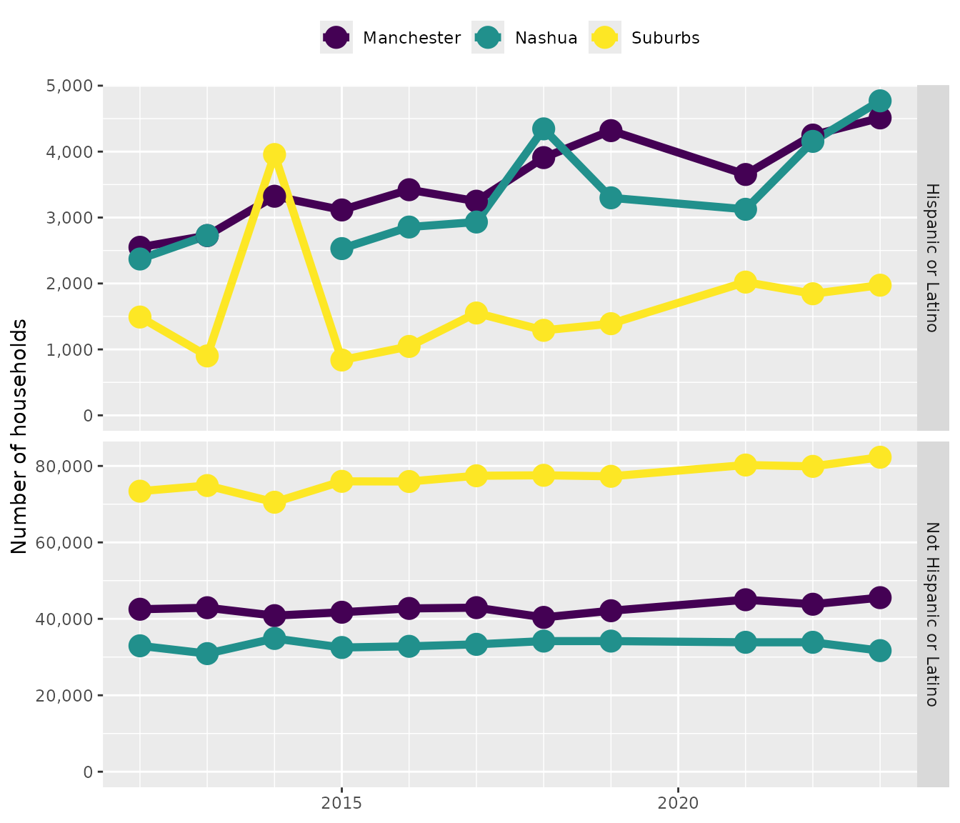
It looks like the number of households is growing, with non-Hispanic households increasing in the suburbs and Hispanic households increasing in the cities.
Analyze
Let’s test this with an ANCOVA. We’ll subtract 2013 from the year so that the intercept estimate gives us the value in 2013, not AD 0.
household_model <- households |>
    dplyr::mutate(
        Year = .data$Year - TEN_YEARS_AGO,
        Location = factor(.data$Location,
                          levels = c("Suburbs",
                                     "Manchester",
                                     "Nashua")),
        Ethnicity = factor(.data$Ethnicity,
                           levels = c("Not Hispanic or Latino",
                                      "Hispanic or Latino"))
    ) |>
    lm(
        Households ~ Year * Ethnicity * Location,
        data = _
    )
I always like to look at the ANOVA table first to get a 10,000 meter view before I try to interpret specific parameters.
household_model |>
    anova() |>
    broom::tidy() |>
    dplyr::mutate(
        dplyr::across(c("sumsq",
                        "meansq"),
                      scales::label_comma(accuracy = 1)),
        dplyr::across("statistic",
                      \(.) signif(., 4)),
        dplyr::across("p.value",
                      \(.) round(., 4))
    ) |>
    knitr::kable(
        align = "lrrrrr"
)| term | df | sumsq | meansq | statistic | p.value |
|---|---|---|---|---|---|
| Year | 1 | 15,150,455 | 15,150,455 | 11.880 | 0.0011 |
| Ethnicity | 1 | 37,914,542,334 | 37,914,542,334 | 29720.000 | 0.0000 |
| Location | 2 | 5,481,169,698 | 2,740,584,849 | 2148.000 | 0.0000 |
| Year:Ethnicity | 1 | 5,758,105 | 5,758,105 | 4.514 | 0.0383 |
| Year:Location | 2 | 4,704,530 | 2,352,265 | 1.844 | 0.1682 |
| Ethnicity:Location | 2 | 6,354,184,575 | 3,177,092,287 | 2491.000 | 0.0000 |
| Year:Ethnicity:Location | 2 | 21,930,681 | 10,965,341 | 8.596 | 0.0006 |
| Residuals | 53 | 67,607,911 | 1,275,621 | NA | NA |
It looks like EVERYTHING is significant, so let’s look at all of the parameters that were in the near-significant range.
household_model |>
    broom::tidy() |>
    dplyr::filter(
        .data$`p.value` < 0.1
    ) |>
    dplyr::mutate(
        dplyr::across(c("estimate",
                        "std.error",
                        "statistic"),
                      \(.) signif(., 4)),
        dplyr::across("p.value",
                      \(.) round(., 4))
    ) |>
    knitr::kable(
        align = "lrrrr"
)| term | estimate | std.error | statistic | p.value |
|---|---|---|---|---|
| (Intercept) | 73410.0 | 614.10 | 119.600 | 0.0000 |
| Year | 753.8 | 95.27 | 7.912 | 0.0000 |
| EthnicityHispanic or Latino | -71850.0 | 868.40 | -82.740 | 0.0000 |
| LocationManchester | -32000.0 | 868.40 | -36.850 | 0.0000 |
| LocationNashua | -40800.0 | 868.40 | -46.990 | 0.0000 |
| Year:EthnicityHispanic or Latino | -723.8 | 134.70 | -5.372 | 0.0000 |
| Year:LocationManchester | -484.8 | 134.70 | -3.599 | 0.0007 |
| Year:LocationNashua | -588.4 | 134.70 | -4.367 | 0.0001 |
| EthnicityHispanic or Latino:LocationManchester | 33350.0 | 1228.00 | 27.160 | 0.0000 |
| EthnicityHispanic or Latino:LocationNashua | 41660.0 | 1272.00 | 32.760 | 0.0000 |
| Year:EthnicityHispanic or Latino:LocationManchester | 611.0 | 190.50 | 3.207 | 0.0023 |
| Year:EthnicityHispanic or Latino:LocationNashua | 751.7 | 194.70 | 3.862 | 0.0003 |
Summarize
The number of households in Hillsborough county overall grew from 2013-2024. The number of Hispanic households was much higher in the two cities than in the suburban parts of the county. This difference became more pronounced over the decade, for two reasons. The number of Hispanic households grew more quickly in Nashua and Manchester than in the suburban areas. The number of non-Hispanic households grew more quickly in the suburbs than in the cities. Isn’t it nice when the visual patterns are corroborated by significant statistics?