Children in Poverty

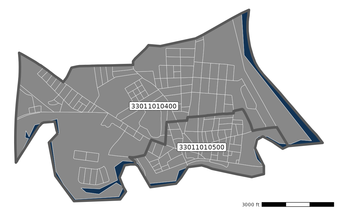
The two tracts are from the northern part of Nashua, NH. Here’s a map:

Families by standard of living

The American Community Survey has a table that categorizes families according to the ratio between their income and the Federal poverty level in their community. Nowadays, the Federal poverty level does not actually represent an income threshold where families really start struggling. It is actually more of a measure of where you are in real danger of starving to death. For that reason, Higher Expectations for Racine County uses three times the Federal poverty level as its threshold for a family-sustaining income. The hercacstables package provides a table, GLOSSARY_OF_STANDARD_OF_LIVING, that describes this classification.

Income ratios from ACS table B17026, classified into standards of living

Variable	Least Poverty Ratio	Greatest Poverty Ratio	Standard of Living
B17026_001E	-999.00	999.00	Everyone
B17026_002E	-999.00	0.50	Unsustainable
B17026_003E	0.50	0.74	Unsustainable
B17026_004E	0.75	0.99	Unsustainable
B17026_005E	1.00	1.24	Unsustainable
B17026_006E	1.25	1.49	Unsustainable
B17026_007E	1.50	1.74	Unsustainable
B17026_008E	1.75	1.84	Unsustainable
B17026_009E	1.85	1.99	Unsustainable
B17026_010E	2.00	2.99	Unsustainable
B17026_011E	3.00	3.99	Family-sustaining
B17026_012E	4.00	4.99	Family-sustaining
B17026_013E	5.00	999.00	Family-sustaining

We use that table and the Census API look up how many families in each tract are in each Census income bracket.

RAW_STANDARD_OF_LIVING <- hercacstables::GLOSSARY_OF_STANDARD_OF_LIVING |>
    dplyr::pull(
        "Variable"
    ) |>
    hercacstables::fetch_data(
        year = 2021L,
        for_geo = "tract",
        for_items = c("010400", "010500"),
        survey_type = "acs",
        table_or_survey_code = "acs5",
        state = 33L,
        county = "011",
        use_key = TRUE
    )

Then, we aggregate to get counts of families experiencing “Unsustainable” and “Sustainable” standards of living.

tract	Family-sustaining	Unsustainable	Everyone	Percent Family-sustaining
010400	957	224	1181	81%
010500	337	633	970	35%

You can see that the economic situations in the two tracts are very different.

Families by children present

We need to go from counts of families to counts of children, so we will next look up how many families in each tract have children. The census has a table for this that reports how many families have no kids, kids under 6, kids 6-17, or both. The hercacstables package has a table, GLOSSARY_OF_FAMILIES_WITH_CHILDREN, that describes the relationship between the ACS variables and the presence/absence of children.

Variable	Adults	Children under 6	Children 6-17
B11003_004E	Married Couple	TRUE	FALSE
B11003_005E	Married Couple	TRUE	TRUE
B11003_006E	Married Couple	FALSE	TRUE
B11003_007E	Married Couple	FALSE	FALSE
B11003_011E	Male householder, no spouse present	TRUE	FALSE
B11003_012E	Male householder, no spouse present	TRUE	TRUE
B11003_013E	Male householder, no spouse present	FALSE	TRUE
B11003_014E	Male householder, no spouse present	FALSE	FALSE
B11003_017E	Female householder, no spouse present	TRUE	FALSE
B11003_018E	Female householder, no spouse present	TRUE	TRUE
B11003_019E	Female householder, no spouse present	FALSE	TRUE
B11003_020E	Female householder, no spouse present	FALSE	FALSE

We can use this table to query the API to get the number of families with children in each of the census tracts that we are interested in. Notice that the only difference between this query and the previous one is which variables we are asking for. The whole point of the hercacstables package is to help you not repeat yourself when you are asking for many different pieces of census information about the same place.

RAW_FAMILIES_WITH_CHILDREN <- hercacstables::GLOSSARY_OF_FAMILIES_WITH_CHILDREN |>
    dplyr::pull(
        "Variable"
    ) |>
    hercacstables::fetch_data(
        year = 2021L,
        for_geo = "tract",
        for_items = c("010400", "010500"),
        survey_type = "acs",
        table_or_survey_code = "acs5",
        state = 33L,
        county = "011",
        use_key = TRUE
    )

We will aggregate the families into “Children Present” and “No Children.”

tract	Children Present	No Children	Total	Percent with Children
010400	460	721	1181	39%
010500	470	500	970	48%

Once again, we see a pretty substantial difference between the two tracts. Reassuringly, the total number of families is the same in both sets of data.

Children per family by poverty level

The last set of raw data that we need is the number of children living in poverty. “But, wait!” you say, “Isn’t that everything we needed in the first place?” That would be true, except that the best we can get from the ACS is a table that has detailed information about parents’ birth origins but only distinguishes three income tiers: less than the Federal poverty level, 1x-2x, and more than 2x the Federal poverty level. The hercacstables package’s table GLOSSARY_OF_CHILDREN_IN_POVERTY describes how the variables in that table map to parental place of birth and kid poverty.

Variable	Least Poverty Ratio	Greatest Poverty Ratio	Standard of Living	Native-Born Parents	Foreign-Born Parents
B05010_004E	-999	1.00	Unsustainable	2	0
B05010_005E	-999	1.00	Unsustainable	0	2
B05010_006E	-999	1.00	Unsustainable	1	1
B05010_008E	-999	1.00	Unsustainable	1	0
B05010_009E	-999	1.00	Unsustainable	0	1
B05010_012E	1	1.99	Unsustainable	2	0
B05010_013E	1	1.99	Unsustainable	0	2
B05010_014E	1	1.99	Unsustainable	1	1
B05010_016E	1	1.99	Unsustainable	1	0
B05010_017E	1	1.99	Unsustainable	0	1
B05010_020E	2	999.00	Mixed	2	0
B05010_021E	2	999.00	Mixed	0	2
B05010_022E	2	999.00	Mixed	1	1
B05010_024E	2	999.00	Mixed	1	0
B05010_025E	2	999.00	Mixed	0	1

Here’s the query to get those data:

RAW_CHILDREN_IN_POVERTY <- hercacstables::GLOSSARY_OF_CHILDREN_IN_POVERTY |>
    dplyr::pull(
        "Variable"
    ) |>
    hercacstables::fetch_data(
        year = 2021L,
        for_geo = "tract",
        for_items = c("010400", "010500"),
        survey_type = "acs",
        table_or_survey_code = "acs5",
        state = 33L,
        county = "011",
        use_key = TRUE
    )

We want 3x the poverty level, so we will lump the “less than 1x” and “1x-2x” tiers into “Unsustainable,” leaving us with the “2x+” tier that mixes both the “2x-3x” tier that we are calling “Unsustainable” and the “3x+” tier that we are calling “Sustainable.”

tract	Mixed	Unsustainable	Children
010400	1037	126	1163
010500	401	322	723

Join the three datasets

Each of the three queries resulted in a data frame where rows correspond to census tracts, so we can join the three results by the “tract” column. We can also remove some of the duplicate columns to end up with just the tract, the number of kids, the number of families, and the percentages of families with children and with sustainable standards of living.

CHILDREN_BY_TRACT <- CHILDREN_IN_POVERTY |>
    dplyr::inner_join(
        FAMILIES_WITH_CHILDREN,
        by = "tract"
    ) |>
    dplyr::inner_join(
        STANDARD_OF_LIVING,
        by = "tract"
    ) |>
    dplyr::select(
        "tract",
        "Children",
        "Mixed",
        "Observed Unsustainable" = "Unsustainable.x",
        "Families" = "Total",
        tidyselect::starts_with("Percent")
    )

This is what that table looks like:

tract	Children	Mixed	Observed Unsustainable	Families	Percent with Children	Percent Family-sustaining
010400	1163	1037	126	1181	39%	81%
010500	723	401	322	970	48%	35%

You can see that, in this case, we did not actually need to pull the number of families with children. If we were doing an even nerdier dive, though, we could use the fraction of families with children to look at poverty across demographics like race or ethnicity.

In this case, though, we just need to multiply the total number of children by the percentage of families that have an sustainable standard of living.

SUSTAINABLE_KIDS <- CHILDREN_BY_TRACT |>
    dplyr::mutate(
        `Expected Unsustainable` = .data$Children * (1 - .data$`Percent Family-sustaining`),
        `Extra Unsustainable` = .data$`Expected Unsustainable` - .data$`Observed Unsustainable`,
        `Sustainable Kids` = .data$Mixed - .data$`Extra Unsustainable`,
        `Percent kids in Sustainable` = .data$`Sustainable Kids` / .data$Children,
        `Expected Sustainable` = .data$Children * .data$`Percent Family-sustaining`
    )

SUSTAINABLE_KIDS |>
    dplyr::select(
        "tract",
        "Children",
        "Percent Family-sustaining",
        "Expected Sustainable",
        "Expected Unsustainable",
        "Mixed",
        "Observed Unsustainable",
        "Extra Unsustainable",
        "Sustainable Kids",
        "Percent kids in Sustainable"
    ) |>
    knitr::kable()

tract	Children	Percent Family-sustaining	Expected Sustainable	Expected Unsustainable	Mixed	Observed Unsustainable	Extra Unsustainable	Sustainable Kids	Percent kids in Sustainable
010400	1163	0.8103302	942.4141	220.5859	1037	126	94.58594	942.4141	0.8103302
010500	723	0.3474227	251.1866	471.8134	401	322	149.81340	251.1866	0.3474227